




At Uniphore we’ve built our approach around small language models: models sized for one job, tuned on conversation data, cheap enough to run on every call. Answering a question like “Did the agent offer to answer further questions?” is exactly that kind of job.
An SLM gets the yes/no right at a fraction of what a frontier model costs, and with lower latency. The explanations are where it breaks down. The SLM tells you why, but it says so differently every time:
- “The agent closed without checking for more questions.”
- “No ‘anything else I can help with?’ before ending.”
- “Customer was transferred before the wrap-up step.”
The first two give the same reason. The third gives a different one. A dashboard can’t tell them apart, and a supervisor shouldn’t have to read 4,000 of them.
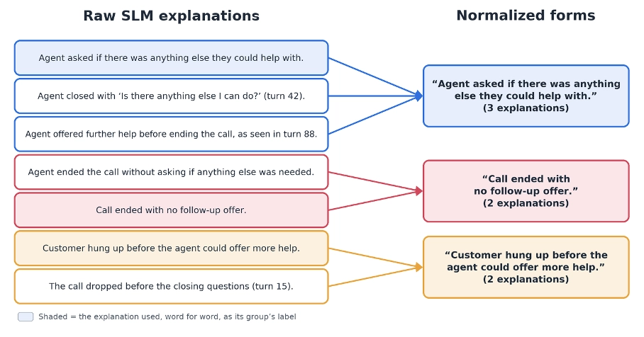
To make explanations useful in aggregate, you have to normalize them: map every explanation to a small set of canonical forms (Figure 1).
The obvious approach, and why we moved away from it
The simplest solution is to ask the SLM again. Keep a running list of normalized forms for each question, and for every new explanation ask the model: “Does this match one of these, or is it something new?”
We built that prototype. It’s consistent and easy to build. But it adds one more SLM generation for every explanation, and at production volume, that cost and latency add up quickly.
So, we reframed the problem. Normalization isn’t a generation task. It’s a clustering task. Group explanations that say the same thing and let one real member of each group stand in as its canonical form. Retrieval and comparison replace generation.
Idea 1: Strip out noise before comparing (Pre-processing)
Explanations often cite where the evidence came from: “…as seen in turns 16, 42, and 96.” Those numbers are provenance, not meaning. Left in, they split otherwise identical explanations into separate clusters.
So, every explanation goes through a narrow rewrite step first: transcript-position references are replaced with a fixed form. For example, these two explanations from different calls:
- “The agent shows empathy and patience towards the customer, as seen in turns 10 and 16.”
- “The agent shows empathy and patience towards the customer, as seen in turns 11, 12 and 19.”
Both become:
“The agent shows empathy and patience towards the customer, as seen in turns N.”
Just as important is what we don’t touch. Numbers, like an eligibility age, a dollar amount, or a contract duration, are part of what the explanation claims, so they stay.
Idea 2: Embeddings propose, NLI decides
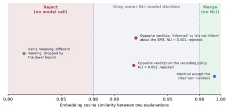
Sentence embeddings are cheap and easy to index, but a single similarity cutoff is unreliable near the decision boundary. Natural language inference (NLI) models read two texts together and are much better at judging whether they say the same thing, but they’re far too expensive to run on every pair. So, we use each where it’s strong:
- Very high similarity (≥ 0.98): merge on the embedding alone.
- Low similarity (< 0.88): reject.
- The gray zone in between: let the NLI model decide, checking both directions.
Figure 2 shows where real pairs fall in these three bands.
The gray zone matters more than you might expect. Most questions are yes/no, so explanations often differ only in polarity:
“The agent informed the client that an SMS was being sent…”
“The agent did not inform the client that an SMS was being sent…”
An embedding model scores that pair at about 0.92 cosine similarity, which is almost identical. The NLI model scores it at about 0.001. This isn’t random noise. It’s a systematic blind spot, and averaging over more neighbors won’t fix it because the neighbors are wrong in the same way. That’s exactly the case the NLI check is there to catch.
With this setup, cost scales with the number of genuinely ambiguous comparisons rather than the number of texts.
Idea 3: Two different jobs, two different paths
Explanations reach us in two ways: a backlog of past ones to sort at the start (we call this seeding), and new ones arriving with every call (online assignment). Each gets its own path, and both use the same store of clusters, as Figure 3 shows.
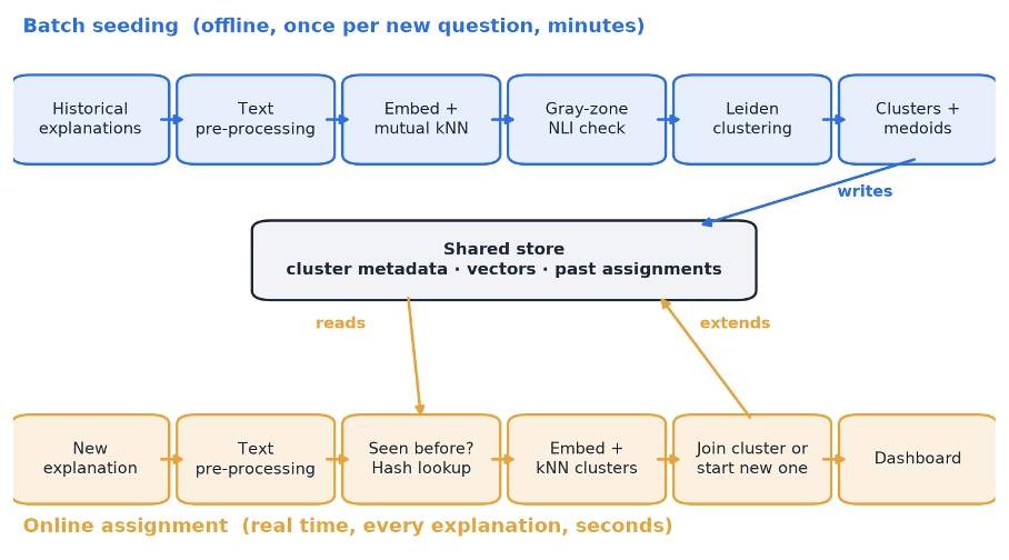
1. Seeding (batch, offline). When a new question is added for normalization of its explanation, we cluster its historical explanations from scratch.
- For small corpora, we run exact pairwise NLI and hierarchical clustering.
- For larger ones, we embed everything, keep only mutual nearest-neighbor edges (so one spurious link can’t chain two unrelated groups together), run the gray-zone NLI check, and partition the graph with Leiden community detection. We never have to guess the number of clusters in advance.
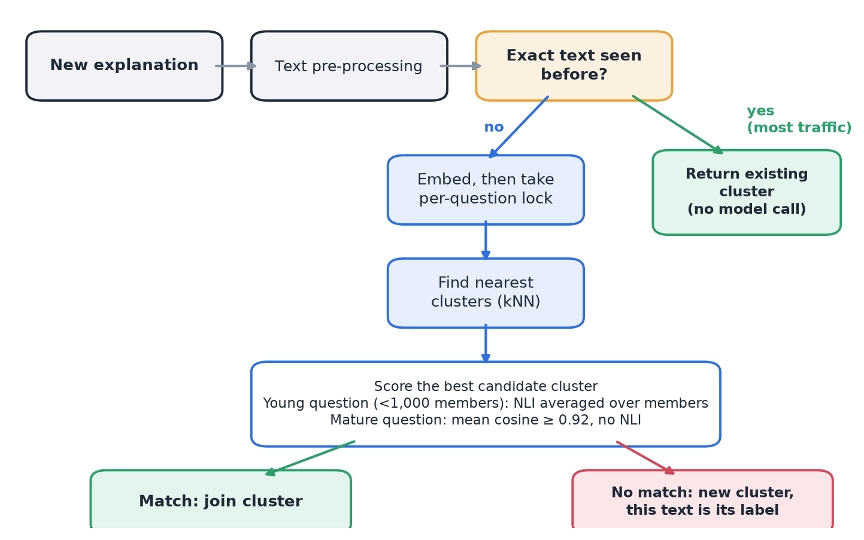
2. Online assignment (real time). Every new explanation has to be placed within seconds, because the dashboard refreshes minutes after a call ends. Figure 4 zooms in on this path, which is the bottom row of Figure 3.
- Most explanations have been seen before. Exact repeats are answered with a hash lookup: no embedding, no model call, no lock.
- New text is embedded, compared against existing clusters, and either joins one or starts a new one.
- A per-question lock prevents two concurrent requests from creating duplicate clusters for the same idea.
Idea 4: Label each cluster with a real explanation
Every cluster needs a label, the one sentence that appears on the dashboard. We use one of the cluster’s own explanations, not something we construct. We considered two alternatives and rejected both:
- The centroid is the average of the cluster’s embeddings. It’s a vector, not a sentence, so there’s nothing to show a user.
- A generated summary reads well, but writing one means calling an SLM, the cost we set out to lower.
A real explanation has neither problem. It’s already written, it costs nothing to pick, and it’s always in the same language as the cluster. Supporting Spanish took no extra work beyond the multilingual models we already use.
How we pick it depends on how the cluster was formed:
- Batch seeding: the mediod, the member closest to the cluster’s center, so the label is the most typical phrasing.
- Online: when a new explanation fits no existing cluster, it starts one and becomes its label.
Once chosen, a label never changes. A dashboard that showed “Call ended with no follow-up offer” last week shows the same words today, so trends stay comparable and no one’s report changes after the fact.
Idea 5: Bounded growth
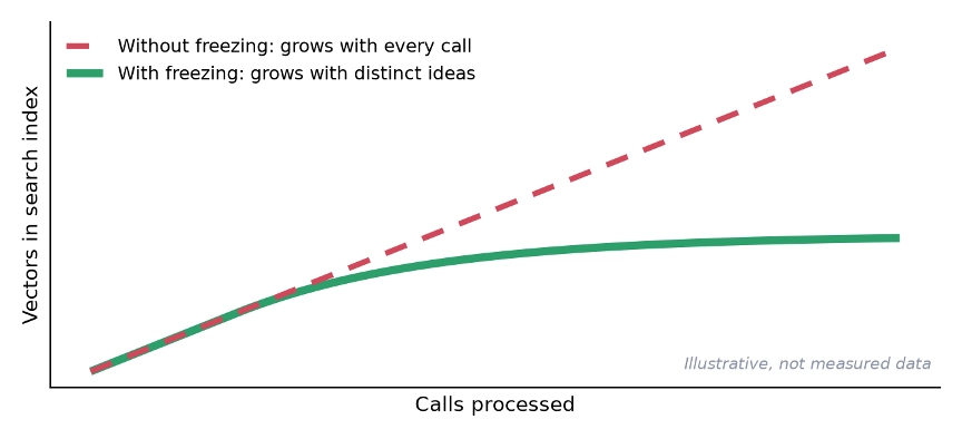
Left unchecked, the searchable index would grow with every call, taking more storage and slowing nearest neighbor lookups. Instead, once a cluster reaches 200 members it’s frozen: new members are still recorded, but they stop adding vectors to the search index. Search state grows with the number of distinct ideas, not the number of calls (Figure 5).
The takeaway
When an SLM’s output needs a second pass, the instinct is to call the SLM again. However, that action is often unnecessary (and expensive). Here, cheap embeddings handle the easy cases, a small NLI model handles the hard ones, a hash table handles repeats, and the final label is simply a real explanation the model already wrote.
The result is normalization that’s consistent, multilingual, and fast enough for production, with almost no extra generation cost.
See what your conversations are trying to tell you. Book a demo.