How Do You Measure an Interruption?

Part 3 of our series on speech recognition in practice. Part 2 reported how our end-of-turn detector compares to leading third-party systems. This post explains how those numbers were produced, and why evaluating endpointing fairly is harder than it looks.

Word error rate (WER) has known problems, but it has an agreed-upon definition. Given a reference transcript and a hypothesis, WER is a well-defined computation once the reference and hypothesis have been normalized. Two labs measuring the same system on the same audio will get the same number.

End-of-turn (EOT) detection is different. Before a system can be scored, three questions need answers. Where exactly does a turn end? What counts as detecting it correctly? And how should the errors be combined into a number that reflects a user’s experience?

None of these questions has a single agreed answer, and every choice moves the results. Deepgram reported that changing only their turn-matching algorithm shifted precision and recall by 3 to 5 points for every system they evaluated [Deepgram, 2025]. Benchmark numbers published without these choices specified are difficult to interpret.

This post states how we decided to measure EOT detection performance. We cover how the ground truth behind the results from Part 2 was built, the four outcomes we score, the metrics we report and the ones we avoid, and the reporting habits that most often distort published comparisons. Along the way we quantify, with our own evaluation data, how much two of these choices move the final numbers.

Building the ground truth

The true EOT location is not directly observable. It is a label, and has to be annotated somehow. Our labels are produced by an automatic pipeline and then verified by human review. The pipeline rests on three ideas.

Use real two-party calls. The source material comprises recordings of real telephone conversations between two speakers, with each speaker on a separate audio channel, sampled at 8 kHz. These are the conditions that reflect our deployment scenarios. Presence of speech in each channel is determined using a Voice Activity Detector.

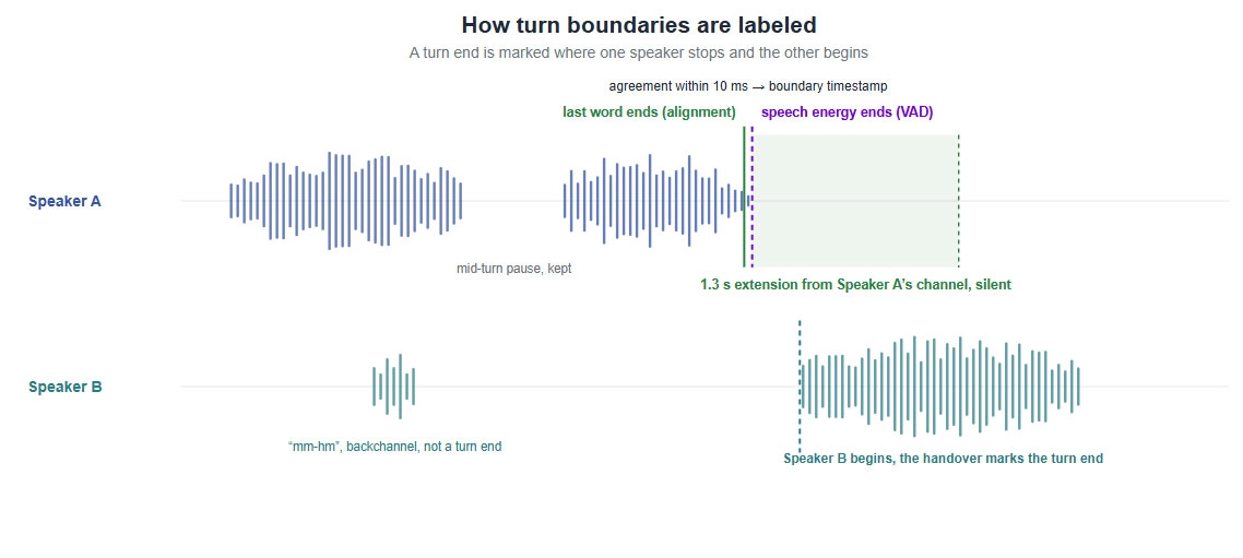
The two channels are what make automatic labeling possible. A turn end is marked where the current speaker stops and the other speaker begins. The handover is itself evidence that the turn was genuinely over.

The evaluation segment is then built from the current speaker’s channel alone, extended 1.3 seconds past the marked end. We chose 1.3 seconds as the post-boundary observation window because it is long enough to expose a meaningful delay after an EOT. Because the channels are separate, the other party’s reply does not appear in this audio, so the detector hears what it would hear in deployment, the speaker’s turn followed by silence. If the speaker’s own channel contains speech inside the extension, the speaker resumed, the pause was not a turn end, and the segment is discarded as a continuation. Backchannels produced by the listener while the speaker is talking, such as “mm-hm,” do not mark a turn end and do not invalidate the segment.

This selection is conservative on purpose. Only unambiguous boundaries become EOT labels. The hard cases remain, because every hesitation and mid-turn pause stays inside the resulting segments. Speakers are also kept disjointed across data splits, so no evaluation speaker appears in training. Figure 1 shows a kept segment with these rules marked, along with the boundary placement described next.

Place the timestamp twice. Latency is measured from the turn-end timestamp, so its placement matters to the millisecond. Human annotators are poor at exactly this. They tend to leave a small gap after the final word, a bias Deepgram documented and corrected with forced alignment [Deepgram, 2025].

We place the timestamp twice, with two independent tools. A voice activity detector (Silero VAD) marks where speech energy ends. Forced alignment of the transcript (WhisperX) marks where the last spoken word ends.

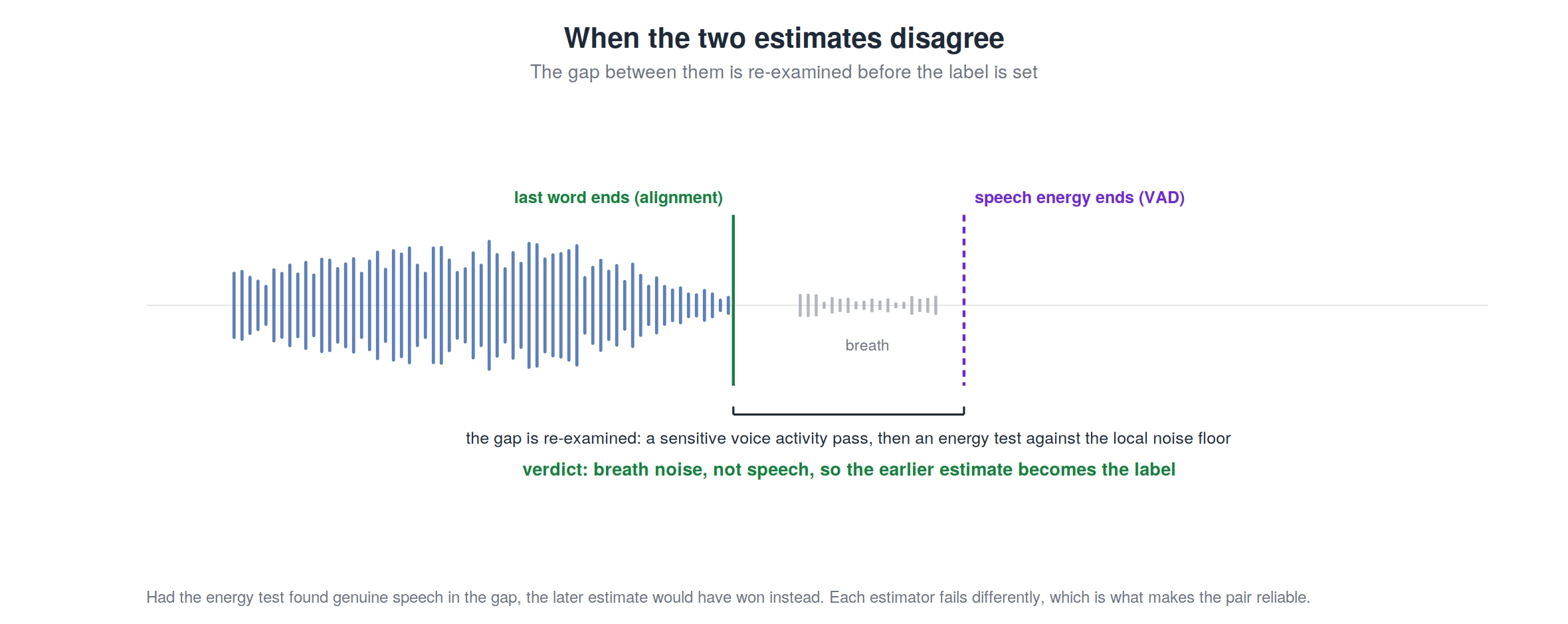
If the two agree within 10 ms, the label is set. If they disagree, the gap between them is examined with a more sensitive voice activity pass, and anything found there is tested against the local noise floor. Real speech in the gap moves the boundary to later. Breath or noise moves it back to the earlier estimate. If alignment fails on a segment, the voice activity estimate is used alone.

The two tools fail in different ways. Energy detection can place the speech end too late when breath sounds or background noise are mistaken for speech, whereas forced alignment can be unreliable when the transcript or alignment is incorrect. Agreement between them is evidence the label is right. Disagreement is a signal to look closer. Figure 2 shows a disagreement being resolved, a breath after the last word that the voice activity detector mistook for speech.

Verify, then measure. The generated labels are checked by human reviewers before use. This divides the work according to each method’s strengths. Automation places timestamps more precisely and more consistently than people can, and people confirm that each boundary is a genuine turn end.

The verified timestamp is the reference for every number in our previous (Part 2) blog post. Latency is measured relative to it, and a detection more than 200 ms preceding it counts as a premature cutoff.

Four possible outcomes

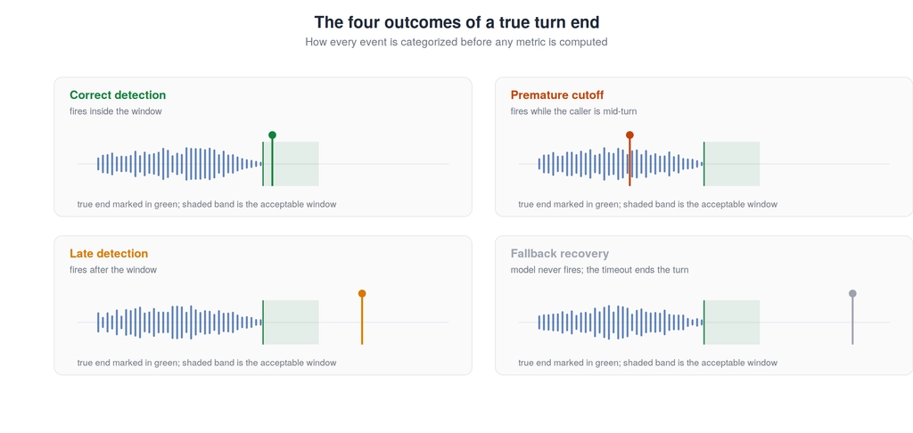
Given labeled conversations, each true EOT results in one of four outcomes. Every event is assigned a category before any aggregate number is computed.

Correct detection. The system fired within the acceptable window around the true turn end. The window opens 200 ms before the true end of speech, the tolerance defined above, and extends through the trailing silence that follows the turn [Shriberg et al].

Premature cutoff. The system fired while the user was still mid-turn. This is the failure speakers experience as being interrupted, and in enterprise deployments it is a costly one. It splits transcripts, degrades intent detection, and forces the speaker to repeat themselves.

Late detection. The system eventually fired, but outside the acceptable window. The user experienced a silent delay. We report these inside the latency percentiles rather than as a separate rate.

Fallback recovery. The model never fired, and a maximum-silence timeout ended the turn instead. Every production endpointing system carries such a fallback, ours included. Deepgram exposes it as a timeout parameter, and AssemblyAI documents a silence fallback in the same role [Deepgram, 2026] [AssemblyAI, 2025].

Figure 3 shows one example of each outcome.

The last category deserves its own section, because conventional aggregate reporting can fail to account for it clearly.

How fallbacks conceal failures

One reporting practice distorts published endpointing numbers more than any other, and a worked example makes it visible.

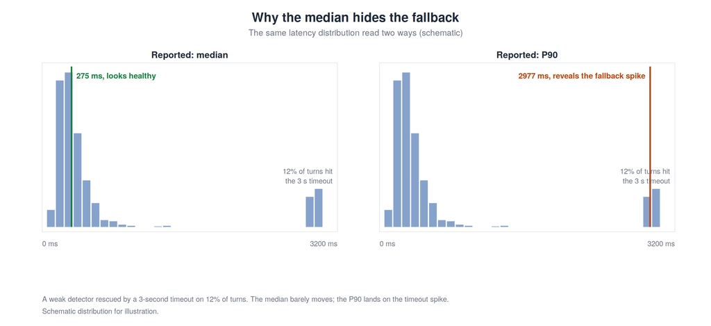
Imagine a detector that recognizes 88 percent of turn ends quickly, at around 250 ms, and simply misses the remaining 12 percent. A 3 second fallback timeout closes the missed turns. Now score this system.

The detection rate looks excellent. Every turn was eventually closed, by the model or by the timeout. If fallback recoveries are counted as detections, the system detects 100 percent of turns.

The median latency looks excellent too. Most turns finish near 250 ms, and the slow 12 percent sit far out in the tail, where the median cannot see them. The reported median stays near 250 ms.

Yet one caller in eight waited three full seconds for a response. That weakness appears in neither headline number. The timeout converted the miss into a detection, and the delay hid beyond the median. Figure 4 shows the same distribution read both ways.

Two reporting rules make the failure visible again.

First, report tail latency. “P90 latency” is the latency of the worst regular moments, and in the example it sits at 3 seconds, exactly on the timeout spike. Callers do not experience the median. They remember the moments the system stalled, and a system that answers quickly nine times and stays silent for three seconds on the tenth is perceived as unreliable. We report P90 latency alongside the median in every comparison and track P99 latency internally.

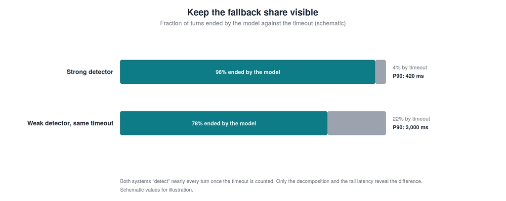
Second, report how often the fallback fired. Whether fallback-recovered turns are counted as detections or as misses matters less than stating which was done, and what fraction of turns needed the fallback. In the example, the single statement that 12 percent of turns were ended by the timeout tells a reader more than either headline number. Figure 5 shows why that share is itself the informative quantity. A detector’s quality is largely a matter of how rarely its safety net is used.

The metrics we report

The categories above reduce to the three quantities reported in Part 2.

Correct endpoint rate is the number of correct detections over true turn ends. We prefer it to precision and recall for a customer deploying EOT, because it answers the operator’s question directly. On what fraction of turns did the system behave correctly?

Premature cutoff rate is reported separately rather than folded into a combined score. The cost of an interruption is not comparable to the cost of latency, and different customers weigh the two differently. A collections workflow and a healthcare workflow do not price an interruption the same way. Publishing the two numbers separately lets each reader apply their own weighting.

Latency, median and P90, is computed over correct detections, measured from the true end of speech.

The numbers we avoid matter as much. We do not publish a single blended score across the trade-off. Any blend assumes a desirable operating point, and comparing systems tuned to different operating points with one number favors whichever system happens to sit closest to that assumption.

For the same reason, third-party comparisons state the configuration used. Every system in this space exposes a parameter that trades cutoffs against speed [Deepgram, 2026], so we sweep the publicly exposed settings and report either the vendor default or the best point we could reach, stated explicitly. A comparison at a single undisclosed configuration is not meaningful.

These choices move real numbers

The claim that evaluation choices matter is easy to make and easy to ignore. Two measurements from our own evaluation in Part 2 show the size of the effect.

Test-set composition. In Part 2, we evaluated Uniphore, Deepgram, and the silence baseline on the full corpus of approximately 19,500 turns. Because of AssemblyAI API limits, we evaluated AssemblyAI (and, for an apples-to-apples comparison, the other systems) on a separate 1,197-turn subset containing comparable numbers of short, medium, and long turns. The two samplings (19.5k and 1.19k) draw from the same corpus, and the subset gives long turns more weight than the natural mix. Table 1 shows the same systems under both samplings.

Table 1: Premature-cutoff rate under two samples from the same corpus.

System	Premature cutoff, full population (%)	Premature cutoff, stratified subset (%)
Uniphore (low-latency point)	6.0	8.5
Deepgram Flux (balanced)	6.1	8.7
Silence baseline (800 ms)	5.9	14.5

Nothing about the systems changed between the columns. Sample composition alone moved every number, by about 2.5 points for the neural systems and by 8.6 points for the silence baseline. Long turns contain more internal pauses, and the baseline that relies on silence alone degrades fastest when they are over-weighted. Note that the shift is not even a uniform penalty. The silence baseline is competitive with Uniphore and Deepgram Flux in the first column and far behind them in the second, so composition can change rankings, not just values.

Scoring rules. On 9.2 percent of the subset’s short utterances, typically backchannels such as “Okay,” AssemblyAI’s API returned a turn-end event with an empty transcript. Is that a detection or a miss? A case can be made either way, and Table 2 shows what each choice does.

Table 2: One scoring decision, two results for the same system on the same audio

Scoring choice	Correct EOT (%)	Premature cutoff (%)
Empty-transcript events counted as misses	76.4	14.5
Those utterances excluded from scoring	84.1	15.9

A single defensible decision moves the system’s correct rate by nearly 8 points, which is larger than the gap between the leading systems in Part 2. Neither choice is wrong. What would be wrong is publishing one of them without saying which. In Part 2 we reported both.

These two effects, together with Deepgram’s finding that turn-matching alone shifts results by 3 to 5 points [Deepgram, 2025], are the foremost reason for calling attention to the issues with EOT detection measurement. Differences of a few points between vendors mean little until the protocol behind them is stated.

Domain matters as much as the model

Part 1 of this series showed accuracy diverging by factors of two to three between conversational telephony test sets and open benchmarks for the same recognition systems. Endpointing is at least as sensitive to domain choice, but for a reason specific to the task.

An endpointing model learns the pause statistics of its training data. Scripted and broadcast speech contains few long hesitations inside turns, so a model trained on it learns that silence means completion. Spontaneous telephone conversation breaks that assumption constantly. Callers pause mid-turn to think, to find documents, or to read off card numbers.

A detector evaluated only on fluent audio has never faced these cases, and its benchmark numbers say little about how it will behave in a contact center. This is why every test set in Part 2 is conversational telephony held out from our training, and why we report per-testset, rather than pooled numbers. Pooling across domains lets strong results on easy audio sources mask weak results on hard speech genres.

The same reasoning applies across languages. Pause behavior, filler words, and prosodic cues at turn ends vary across languages and regional accents, so we evaluate each language on its own conversational test sets rather than assuming results carry over.

Three practices worth adopting

Evaluation practice in endpointing today resembles ASR evaluation before common test sets existed. Each vendor reports self-selected numbers under undisclosed protocols. Full standardization may take time, but published endpointing results would be substantially easier to compare if evaluations consistently did three things:

• Describe ground truth: State how candidate turn boundaries and final end-of-speech timestamps were determined, including any forced-alignment correction.
• Report latency tails: Report median and P90 latency, rather than median latency alone.
• Disclose the operating point: State each system’s endpointing configuration and fallback timeout, and separately report model detections and fallback recoveries.

The next post in this series will return to the model itself. In it, we will examine how end-of-turn detection behaves across languages, and whether a detector trained in one language has learned anything that a second language can use.

References

- Deepgram (2025). Evaluating End-of-Turn (Turn Detection) Models. https://deepgram.com/learn/evaluating-end-of-turn-detection-models
- Deepgram (2026). End-of-Turn Detection Parameters, Flux Documentation. https://developers.deepgram.com/docs/flux/configuration
- AssemblyAI (2025). Introducing Universal-Streaming. https://www.assemblyai.com/blog/introducing-universal-streaming
- Uniphore (2026). Automatic Speech Recognition in Practice (Part 1 of this series).
- Uniphore (2026). Knowing When to Speak (Part 2 of this series).
- Shriberg et al. (2001). Observations on overlap: findings and implications for automatic processing of multi-party conversation. Proc. of Eurospeech, pp. 1359-1362.