Knowing When to Speak

This is part 2 of our series on speech recognition in practice. Part 1, Automatic Speech Recognition in Practice, described how modern ASR systems are designed and benchmarked. This post covers the problem that begins where transcription ends. How does a voice agent decide that a speaker has finished?

In human conversation, the gap between one speaker finishing and the next speaker starting is very short. Sacks, Schegloff, and Jefferson observed in their early work on conversational structure that most transitions between speakers happen with no gap and no overlap, or only a slight one [Sacks et al., 1974]. Later measurements confirmed this across languages. In a study of question-answer pairs in ten unrelated languages, the most common gap between question and answer was between 0 and 200 milliseconds in every language, and the mean gap was under 500 milliseconds in all of them [Stivers et al., 2009].

These gaps are too short to be explained by reaction alone. Planning even a simple spoken response takes about 600 milliseconds, so a listener who waited for silence before starting to plan could not answer within 200 milliseconds [Levinson and Torreira, 2015]. The conclusion drawn in that work is that listeners do not detect the end of a turn after it happens. They predict it from cues in the ongoing speech, and they prepare their response before the speaker has finished.

A voice agent has to make the same judgment, many times per call, and it has no such predictive ability unless we build it. The task is called endpointing, or end-of-turn (EOT) detection. It can fail in two directions. If the system decides too early, it interrupts a caller who paused to look up a policy number. If it decides too late, every exchange in the conversation carries an extra silent delay before the agent responds, and the conversation feels slow.

At Uniphore, endpointing is built into the streaming ASR stack rather than added on top of it. This post explains why the problem is hard, what information a pause carries, how the industry has converged on a small set of designs, the choices behind our own detector, and how it compares to leading third-party systems on conversational telephone audio.

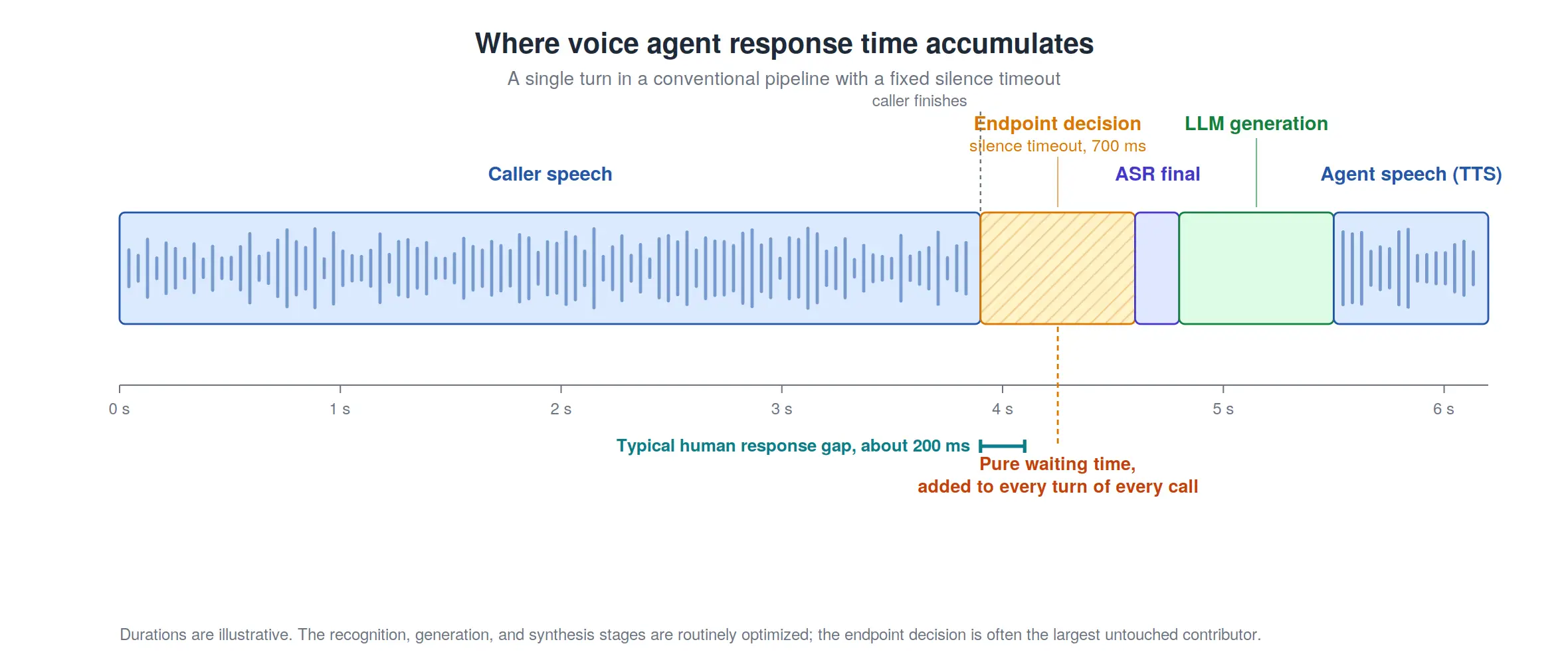
Where response latency comes from

When teams measure the responsiveness of a voice agent, they usually measure the visible components. Recognition speed, language model generation, and speech synthesis are all profiled and optimized, and each has improved in recent years.

A less visible component often adds more delay than any of them. Before the language model can start generating, the system must decide that the user has finished speaking. In a conventional pipeline this decision is made by a silence timeout. A voice activity detector monitors the audio, and once non-speech has lasted a fixed duration, commonly between 500 and 1000 milliseconds, the turn is declared over. Because the timeout is a waiting period, its full length is added to the response time of every turn in every call. A pipeline with a 700 millisecond timeout adds 700 milliseconds of silence to each exchange before recognition, generation, or synthesis contribute anything. Compared to the 200 millisecond gaps of human conversation, this is where much of the perceived slowness comes from.

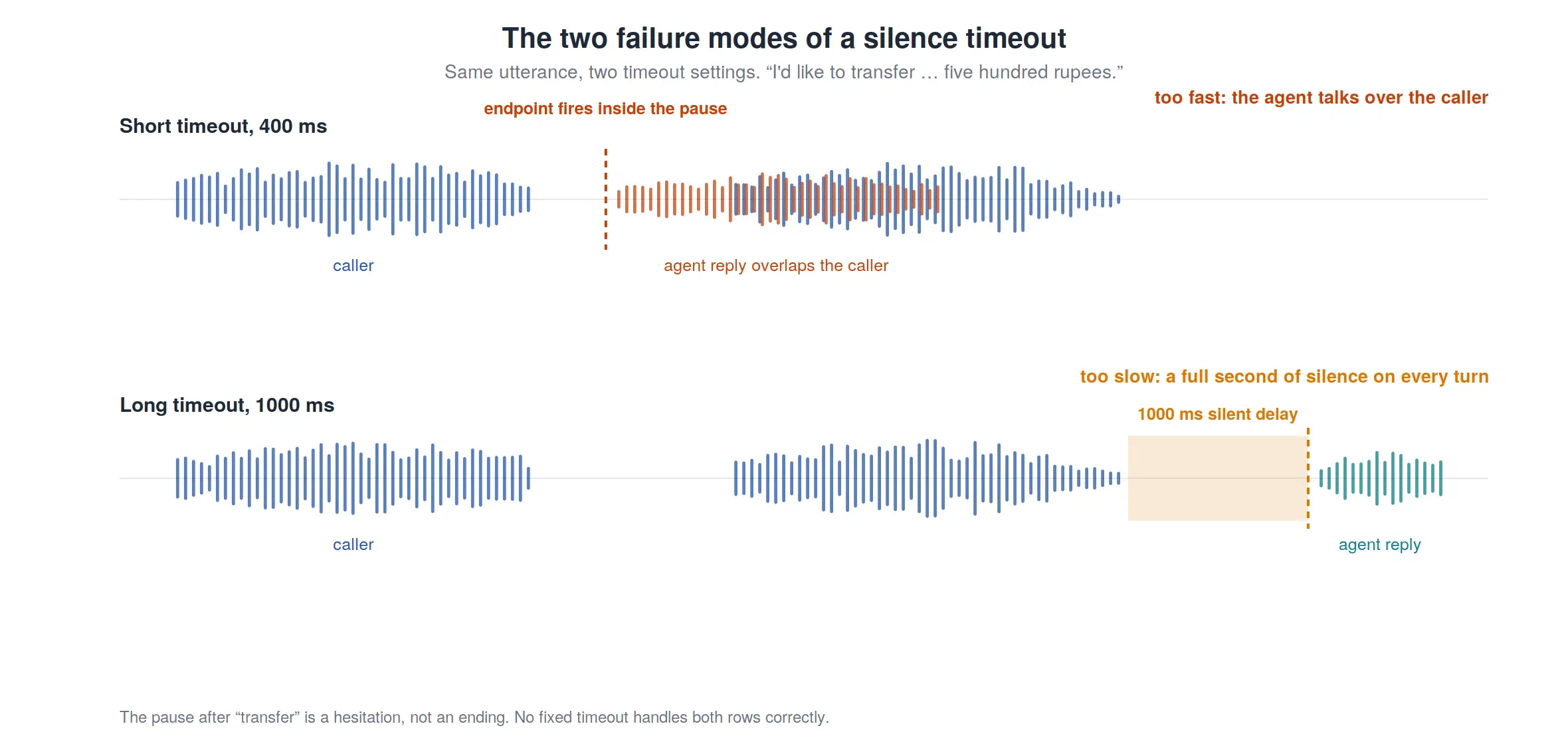
Shortening the timeout does not fix this. It moves the failure to the other side. Spontaneous speech contains many pauses inside turns. Callers hesitate, correct themselves, and read out numbers digit by digit. A caller may say “I want to transfer” and then pause for two seconds while checking the amount. One published analysis of conversational speech found that nearly a quarter of pause-bounded speech segments were continuations of the same turn rather than turn endings [AssemblyAI, 2025a]. A short timeout fires inside these pauses, and the agent starts speaking while the caller is still mid-turn. In an enterprise deployment this has costs beyond the moment itself. The interrupted caller repeats the utterance, the transcript is split across turn boundaries, intent classification receives partial inputs, and handling time goes up.

The underlying problem is that silence duration alone cannot answer the question being asked of it. Whether a 600 millisecond pause means the turn is over depends on what was said before the pause and how it was said. A fixed threshold is therefore too slow for turns that ended cleanly and too fast for turns that contain hesitation, at the same time. The rest of this post is about the additional evidence that resolves this ambiguity, and how current systems use it.

What a pause contains

A pause is not one kind of event. When speech stops, the speaker may have finished the turn, may be hesitating mid-thought, or may be doing something else, such as finding a document. The evidence for telling these apart comes from three separate parts of the signal, and the strengths and weaknesses of each explain the structure of every endpointing system built so far.

Acoustic evidence. The most basic information is whether speech energy is present, which is what a voice activity detector measures. This establishes that a pause has started and how long it has lasted. Its reliability drops under contact center audio conditions. Telephone networks carry audio sampled at 8 kHz, which preserves frequencies only up to about 4 kHz and loses the higher-frequency detail present in wideband recordings. Add background noise, cross-talk, and hold music, and even the basic question of whether anyone is speaking becomes error-prone. Every later decision inherits those errors.

Prosodic evidence. How the last stretch of speech was produced carries information about whether more is coming. Speakers ending a turn tend to produce falling pitch and a lengthened final syllable. Speakers who intend to continue tend to hold their pitch level and often end the speech region with a filled pause such as “um.” These patterns have been used for automatic endpointing for more than two decades. Ferrer, Shriberg, and Stolcke showed that classifiers using prosodic features, mainly pitch and duration patterns before a pause, could identify utterance endpoints earlier than waiting on pause duration alone, without increasing the error rate [Ferrer et al., 2003]. Prosodic cues are available directly from the audio, before any transcript exists, which makes them useful for latency. Their weakness is variability. They are harder to read on narrowband noisy audio, and they differ across speakers, accents, and languages.

Semantic evidence. What was said constrains whether the thought is complete. “My new address is” is an unfinished sentence, and a listener expecting the address will wait through a long pause without responding. “My new address is 14 Lake View Road” is a complete sentence, and even a short pause after it invites a reply. Semantic evidence answers the completion question most directly, but it has two costs. It only becomes available through recognition, so it arrives later than the audio and inherits transcription errors. It is also not conclusive by itself, because a complete sentence is often followed by more, as in “I want to cancel my subscription. Also, one more thing.”

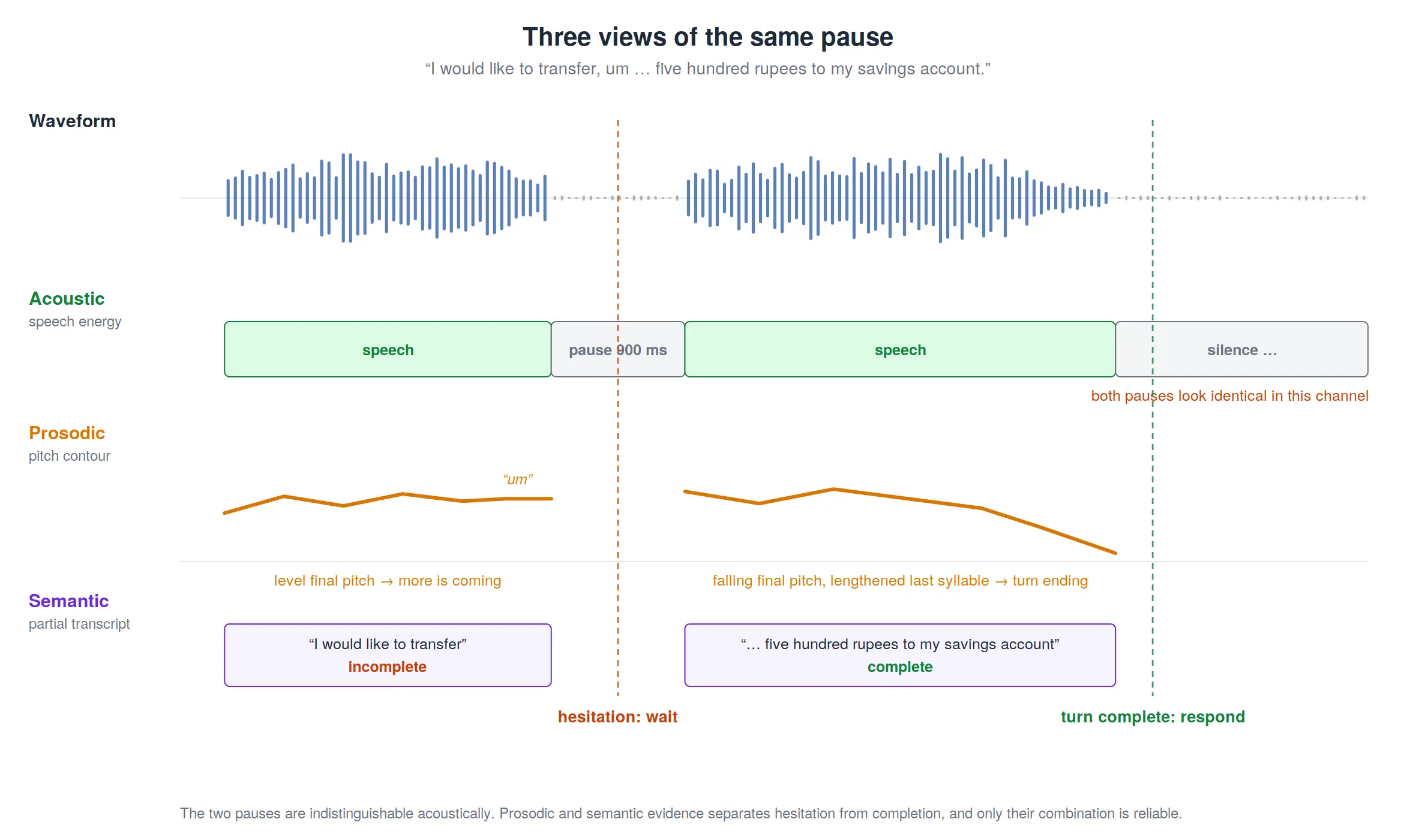
No single channel is enough. Acoustic evidence cannot separate hesitation from completion. Prosodic evidence is informative, but it is least reliable on narrowband, noisy telephone audio, which is exactly the audio that enterprise systems receive. Semantic evidence arrives late, inherits recognition errors, and does not resolve every case. Figure 4 makes the point with four short utterances, two where the channels agree and two where only their combination gives the right answer.

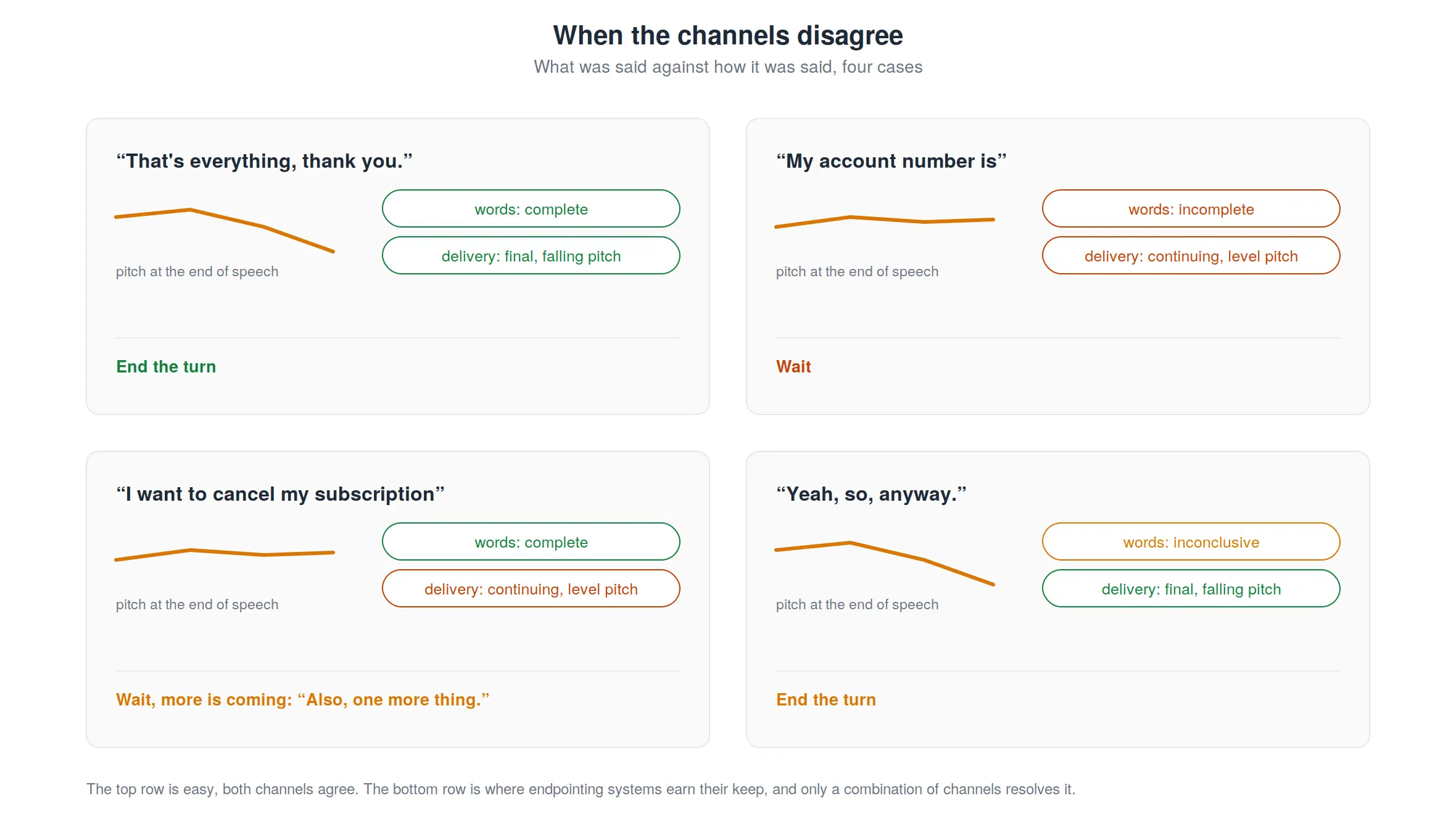
Human listeners combine all three continuously, which is what makes the predictive turn-taking described in the introduction possible. The engineering question, and the main way systems differ, is how to combine the three channels into one streaming decision under a strict latency budget. The next section surveys the answers currently in production.

How the industry has converged

Part 1 of this series observed that the apparent variety of commercial ASR systems hides a small number of shared designs. The same is true of endpointing. Current production systems fall into four designs, and each can be read as a different answer to the combination question above.

Silence-based endpointing is the legacy default. A voice activity detector is paired with a timeout, sometimes with an auxiliary model that adjusts the timeout length. The design uses only the acoustic channel. It is simple and language-independent, and it survives as the fallback layer inside nearly every modern system, but its limits are the ones described in the previous section.

Text-based turn detectors add the semantic channel. A small language model (SLM) runs over the streaming transcript and scores whether the utterance so far reads as complete. The best known example is LiveKit’s open turn detector, a compact transformer distilled from a larger model for fast CPU inference. It estimates end-of-utterance probability from the transcribed conversation and is used to suppress interruptions that a VAD alone would cause [LiveKit, 2024]. The design gains real semantic judgment, but it pays the costs identified above. The model sees the words but not how they were spoken, and because it runs after the recognizer, it inherits transcription latency and transcription errors.

Audio-based turn classifiers make the opposite choice. Small models such as Pipecat’s Smart Turn and Krisp’s turn prediction models take audio directly and classify whether the current turn is complete, using the prosodic evidence that text-based detectors discard [Krisp, 2026]. They need no transcript and run with low latency on CPU. Their limitation is the reverse of the text-based design. They observe how the caller spoke but not what was said, so an utterance that sounds finished but is not grammatically complete can produce a false ending.

Integrated ASR and endpointing models put the turn decision inside the recognizer itself. The argument is that the recognizer is the one component with access to all three channels at once. Deepgram’s Flux is built on this principle. It replaces separate recognition, voice activity detection, and endpointing components with a single model that emits turn events alongside transcripts. Deepgram reports that this integration reduced agent response latency by 200 to 600 milliseconds relative to pipeline approaches and reduced false interruptions by about 30 percent in their evaluations [Deepgram, 2025a]. AssemblyAI’s Universal-Streaming takes the same direction, integrating end-of-turn detection into the streaming recognizer and combining acoustic and semantic features with a silence fallback [AssemblyAI, 2025b]. Integration also removes a coordination problem that pipelines have. When a separate turn detector and a separate recognizer disagree, for example when a turn-end event arrives while the transcript is still partial, the application around them has to resolve the conflict, and these disagreements occur most often in the hardest cases [Deepgram, 2025b].

Two further developments extend this picture. The first is the use of graded endpoint confidence to overlap computation. When an integrated model is moderately confident that a turn has ended, downstream language model processing can start early and be discarded if the caller resumes. Deepgram exposes this as eager end-of-turn events [Deepgram, 2026]. The second is the arrival of speech-native language models, discussed in Part 1, which handle turn-taking as part of general conversational modeling rather than as a separate detection task. Both point the same way. Recognizing speech and deciding when to respond are becoming harder to separate, much as acoustic, pronunciation, and language models merged in ASR a decade earlier.

Endpointing inside the recognizer, the Uniphore approach

Uniphore builds conversational AI for enterprise contact centers, and this setting makes the endpointing problem harder in specific ways. The audio is narrowband telephony with real-world noise. Callers vary widely in accent and speaking style. The speech is spontaneous and task-oriented, with frequent hesitation, self-correction, and long number sequences such as policy numbers and payment references, which are exactly the utterances most likely to contain long pauses inside a turn. Finally, the cost of an error differs by deployment. A collections workflow may accept an occasional early response in exchange for speed. A healthcare workflow may accept slower responses but must not interrupt a patient describing symptoms. A detector built and evaluated on clean, wideband English audio does not transfer well to this setting. This matches the domain sensitivity we documented for recognition accuracy in Part 1.

Our design follows from these constraints, and it builds on our previously published work on integrating endpointing into streaming transducer ASR [–, 2026].

The endpoint decision is made inside the streaming recognizer. As described in Part 1, our real-time models are Zipformer encoders trained with transducer objectives. The endpoint decision is computed by the same stack, over the same frames, in the same streaming pass as recognition. The practical reason is access to information. A streaming recognizer already tracks, frame by frame, whether speech is currently being decoded, so the acoustic evidence of a pause does not need to be recomputed by a separate voice activity detector running on raw audio. Making the decision inside the recognizer puts all three evidence channels in one component with no added latency. This is the same argument that motivates the integrated designs described above.

The decision combines acoustic, prosodic, and semantic evidence. The detector uses the length of the pause, prosodic cues such as intonation in the speech leading into it, and the semantic state of the ongoing recognition. As noted in Part 1, intonation in particular lets the system separate a mid-turn hesitation from a completed turn before any fixed silence threshold could. This is what prevents the early responses that silence-only designs produce on hesitant speech.

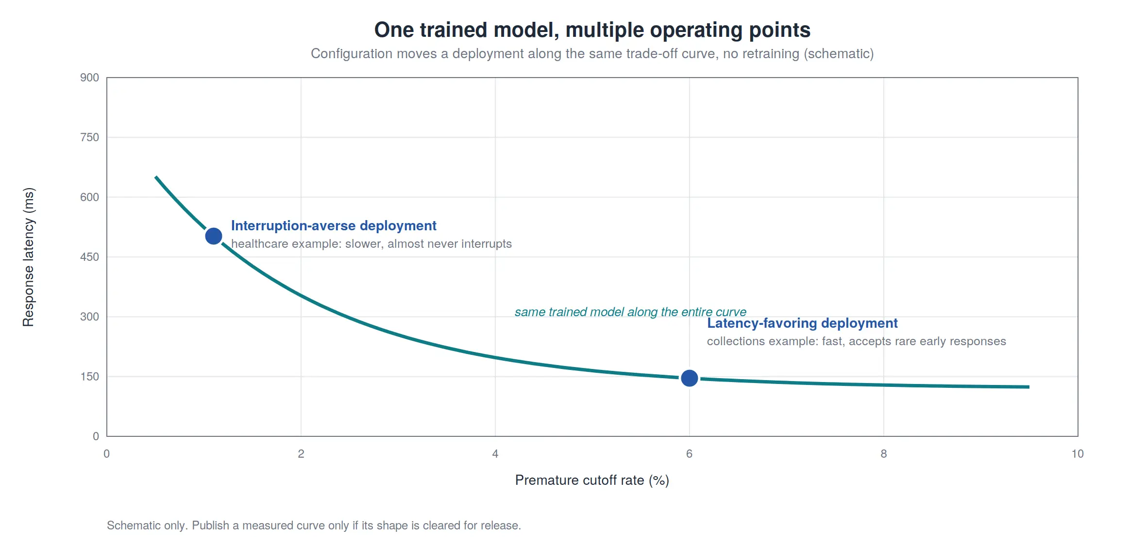
A single model supports multiple operating points. Because deployments weigh interruptions against latency differently, the detector is designed to be tuned per deployment rather than retrained. The same trained model runs in a latency-favoring configuration for one customer and an interruption-averse configuration for another. In practice this turns a modeling property into an operational one. Supporting a customer with different conversational norms becomes a configuration task rather than a training project, which matters at the scale of enterprise onboarding. Figure 5 sketches the idea.

The specific way the evidence channels are combined at decision time, and the training procedure that makes the combination reliable in production will be described in a later post in this series. What we report now is how the resulting system performs.

Putting it to the test

Following the methodology of Part 1, we evaluate on held-out conversational telephony test sets that reflect the traffic our deployments actually process, and we compare against leading third-party systems accessed through their public streaming APIs. The evaluation covers about 32 hours of audio and roughly 19,500 turns across 15 English test sets, spanning regional accent variants and several enterprise domains. Evaluating endpointing fairly involves several non-obvious choices, in how ground truth is built, in how detections are matched to turns, and in how errors are aggregated. The next post in this series is devoted entirely to that methodology. Here we define the reported quantities briefly and present the results.

Correct endpoint rate. The fraction of true turn endings that the system detected within an acceptable window. A detection up to 200 ms before the true end of speech is tolerated. Correct and premature rates do not always sum to 100 percent, because a small fraction of turns are never detected within the window and are counted as misses.

Premature cutoff rate. The fraction of turns on which the system fired more than 200 ms before the true end of speech, while the caller was still mid-turn. This is the failure a caller experiences as being interrupted.

Latency, median and P90. The time from the true end of speech to the endpoint decision, computed over correctly detected turns. We report the 90th percentile alongside the median because a system that is fast on most turns but occasionally adds a multi-second delay is still experienced as slow. Deepgram’s evaluation work makes the same argument for reporting the tail of the latency distribution [Deepgram, 2025c].

Uniphore was run at its low-latency operating point. Deepgram Flux was run at its balanced setting. AssemblyAI Universal-Streaming was run at a balanced setting using its public parameters, an end-of-turn confidence of 0.7 and a minimum silence of 560 ms. The silence baseline is a voice activity detector with a fixed timeout. All third-party systems were accessed through their public streaming APIs in July 2026.

Table 1: Overall results on the full population, about 19,500 turns across 15 test sets

System	Correct EOT (%)	Premature cutoff (%)	Median latency (ms)	P90 latency (ms)
Uniphore (low-latency point)	92.7	6.0	220	400
Deepgram Flux (balanced)	92.3	6.1	230	980
Silence baseline (800 ms)	94.1	5.9	890	2080

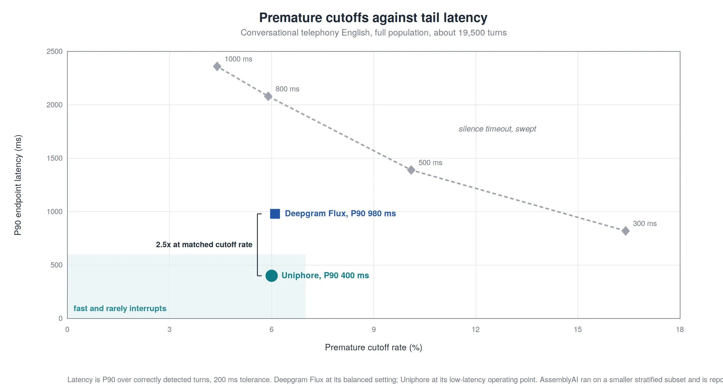
The silence baseline in Table 1 was tuned so that its premature cutoff rate matches the neural systems, which makes the latency comparison direct. Figure 6 additionally sweeps the timeout across its useful range, from 300 ms to 1000 ms, to show that no other setting escapes the trade-off.

AssemblyAI’s public API limited us to a smaller evaluation, so it is reported separately. Its account-level concurrency limits made streaming the full corpus impractical, and we instead ran a 1,197-turn subset, stratified across ten duration bins, with all four systems evaluated on exactly the same turns. Because the stratification gives long turns more weight than the natural mix, this subset is harder than the full population, which is why every system’s numbers are slightly worse in Table 2 than in Table 1. Numbers from Table 2 should therefore be compared only within Table 2.

Table 2: Duration-stratified subset, 1,197 turns, all systems on identical audio

System	Correct EOT (%)	Premature cutoff (%)	Median latency (ms)	P90 latency (ms)
Uniphore (low-latency point)	90.1	8.5	210	390
Deepgram Flux (balanced)	89.6	8.7	210	980
AssemblyAI Universal-Streaming (balanced)	76.4	14.5	150	550
Silence baseline (800 ms)	85.5	14.5	880	2018

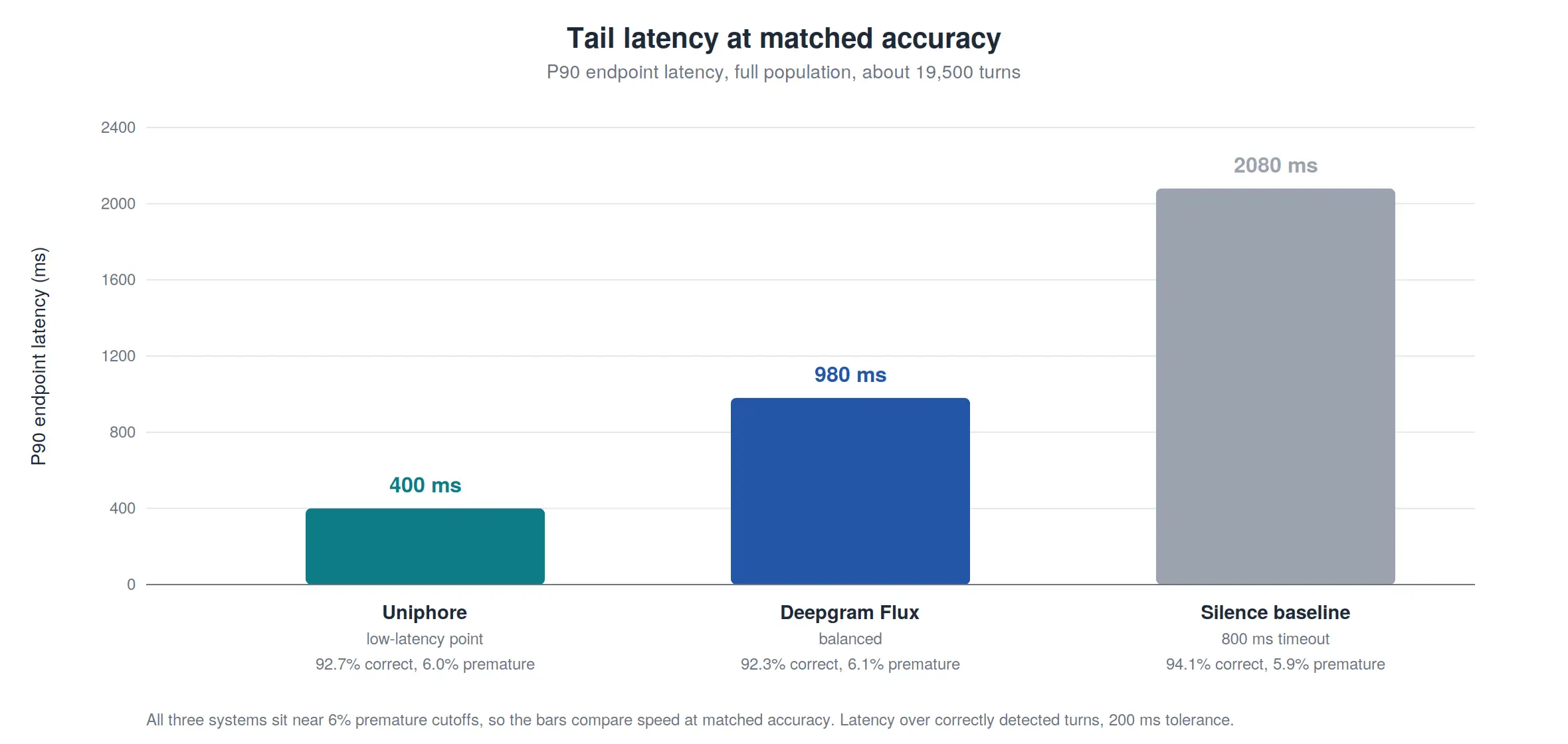
Three results stand out. First, on the full population (Table 1), at a matched premature cutoff rate of about 6 percent, Uniphore and Deepgram Flux are equivalent on correct endpoint rate and median latency, but they separate sharply in the tail. Uniphore’s P90 latency is 400 ms against 980 ms for Flux, a factor of about 2.5. Since the tail of the latency distribution is what callers remember, this is the difference between a conversation that occasionally stalls and one that does not. Figure 7 isolates this comparison.

Second, the silence baseline is dominated on both axes at every timeout value. Tuned to match the neural systems on premature cutoffs (800 ms), it is roughly four times slower at the median and five times slower at P90. Tuned toward their latency (300 ms), its premature cutoff rate rises to 16.4 percent, close to one interrupted caller in six. No fixed timeout reaches both the accuracy and the speed of a neural endpointer, which is the quantitative form of the argument made at the start of this post.

Third, on the stratified subset (Table 2), AssemblyAI’s balanced setting is the fastest system at the median (150 ms) but fires prematurely on 14.5 percent of turns, about 1.7 times the rate of Uniphore and Flux on identical audio. Part of its lower correct rate has a separate cause. On 9.2 percent of the subset’s short utterances, typically backchannels such as “Okay,” it emitted an end-of-turn event with an empty transcript, which our scoring counts as a miss. Excluding those turns, its balanced setting scores 84.1 percent correct with a 15.9 percent premature cutoff rate. We report both views for completeness.

The usual caveats from Part 1 apply here as well. No system wins on every individual test set, and the aggregate numbers above average over sets of varying difficulty. Training data and model scale differ across systems, third-party systems were evaluated at the settings stated above and other settings trade the same quantities differently, and results on other domains will vary with training distribution rather than architectural capability.

Conclusion

Endpointing connects everything this series has discussed so far. It uses the recognizer’s acoustic representations, it depends on the recognizer’s text output, and it sets the starting time for every component after it. The industry’s move toward integrated designs reflects a shared conclusion. The question “has this speaker finished” is neither purely acoustic nor purely linguistic, and systems answer it well only when they stop treating it as a separate problem. Human conversation, with its 200 millisecond transitions built on prediction, remains the reference point for how good these systems can become.

The comparisons above also raise a question: when we report that a system interrupted a caller, how do we know? Building reliable ground truth for turn endings, and choosing metrics that do not hide failure modes, is a substantial problem on its own, and it is the subject of the next post in this series.

References

- Sacks, H., Schegloff, E. A., & Jefferson, G. (1974). A Simplest Systematics for the Organization of Turn-Taking for Conversation. Language, 50(4), pp. 696–735.
- Stivers, T., Enfield, N. J., Brown, P., Englert, C., Hayashi, M., Heinemann, T., Hoymann, G., Rossano, F., de Ruiter, J. P., Yoon, K.-E., & Levinson, S. C. (2009). Universals and Cultural Variation in Turn-Taking in Conversation. Proceedings of the National Academy of Sciences, 106(26), pp. 10587–10592. https://www.pnas.org/doi/10.1073/pnas.0903616106
- Levinson, S. C., & Torreira, F. (2015). Timing in Turn-Taking and Its Implications for Processing Models of Language. Frontiers in Psychology, 6:731. doi:10.3389/fpsyg.2015.00731
- Ferrer, L., Shriberg, E., & Stolcke, A. (2003). A Prosody-Based Approach to End-of-Utterance Detection That Does Not Require Speech Recognition. Proc. IEEE ICASSP 2003, Hong Kong, vol. I. https://www.sri.com/wp-content/uploads/2021/12/a_prosody-based_approach_to_end-of-utterance_detection_th.pdf
- Anandh, C., Pandia Durai, K., Prakash, J., Arumugam, M., Hacioglu, K., Dubagunta, S. P., Stolcke, A., Venkatesan, S., & Ganapathiraju, A. (2025). Improving Endpoint Detection in End-to-End Streaming ASR for Conversational Speech. arXiv:2505.17070. https://arxiv.org/abs/2505.17070
- AssemblyAI (2025a). How Intelligent Turn Detection (Endpointing) Solves the Biggest Challenge in Voice Agent Development. https://www.assemblyai.com/blog/turn-detection-endpointing-voice-agent
- AssemblyAI (2025b). Introducing Universal-Streaming. https://www.assemblyai.com/blog/introducing-universal-streaming
- LiveKit (2024). Using a Transformer to Improve End-of-Turn Detection. https://blog.livekit.io/using-a-transformer-to-improve-end-of-turn-detection
- Krisp (2026). A Solution to Turn-Taking and Interruption Prediction in Voice AI. https://krisp.ai/blog/voice-ai-turn-taking-interruption-prediction/
- Deepgram (2025a). Introducing Flux: Conversational Speech Recognition. https://deepgram.com/learn/introducing-flux-conversational-speech-recognition
- Deepgram (2025b). Fluxing Conversational State and Speech-to-Text. https://deepgram.com/learn/fluxing-conversational-state-and-speech-to-text
- Deepgram (2025c). Evaluating End-of-Turn (Turn Detection) Models. https://deepgram.com/learn/evaluating-end-of-turn-detection-models
- Deepgram (2026). Optimize Voice Agent Latency with Eager End of Turn. https://developers.deepgram.com/docs/flux/voice-agent-eager-eot
- Uniphore (2026). Automatic Speech Recognition in Practice (Part 1 of this series). https://www.uniphore.com/blog/automatic-speech-recognition-in-practice/